Using RQDA for Qualitative analysis

Diarmuid O'Briain, diarmuid@obriain.com
30/09/2018, version 1.4

---

• Introduction
  • Qualitative Content Analysis
  • Coding
• Using RDQA()
  • Starting RQDA()
    • Add the RQDA library
    • Create a Project
    • Import source files to the project
  • Coding
    • Inductive approach
    • Deductive approach
  • Reviewing Coding
  • Reviewing the coded blocks
  • Visualising categories
    • Installing d3Network
    • Visualising Categories
  • Summary

---

Introduction

The r-project text is a free software environment for statistical computing and graphics. It has is a network of ftp and web servers around the world that store identical, up-to-date, versions of code and documentation for R called the Comprehensive R Archive Network (CRAN). One of the packages R Qualitative Data Analysis (RQDA) is a free software for qualitative text and PDF document analysis.

It is particularly useful for inductive thematic analysis however for deductive analysis it is necessary to upload Categories and Codes one by one. RQDA Code Builder resolves this.

This document demonstrates how to use RQDA() and the RQDA Code Builder on a GNU/Linux platform. R and RQDA() can be used on other platforms like Microsoft Windows and as the RQDA Code Builder is Python3 based it can easily be adapted for other platform implementations.

It will be necessary to have python3 installed on the platform. Use the Software Manager for your GNU/Linux flavour or install using apt from the shell.

  $ sudo apt-get install python3
  $ sudo apt-get install python-yaml
  

Confirm the install and the version of python3.

  $ python3 --version
    Python 3.5.2
  

Qualitative Content Analysis

Qualitative Content Analysis follows a procedure:

1. Deciding the research question
2. Selecting material
3. Building a coding frame
4. Segmentation
5. Trial coding
6. Evaluating and modifying the coding frame
7. Main analysis
8. Presenting and interpreting the findings.

  Uwe Flick. An Introduction to Qualitative Research. 5th Edition. ISBN: 1446297721, 9781446297728. SAGE, 2014.
  

Coding

Assuming that steps 1 and 2 are completed and the next step is the building of a coding frame. There are two approaches, inductive and deductive.

The inductive approach has codes extracted directly from the source data. As the researcher reads through each source file (interviews, papers, etc..), he or she highlights key lines and creates a code for it. These codes are added and modified as the researcher reads through all the source material. The codes are then bundled into codes of common category. RDQA() is very suitable for this approach.

The deductive approach involves the researcher developing codes and categories in advance, in a scheme. These codes are then applied to the source data. As RDQA() expects codes to be added one by one through the graphical interface this is difficult. Application of the rqda_code_builder.py program described here helps to fix this.

Using RDQA()

Starting RQDA()

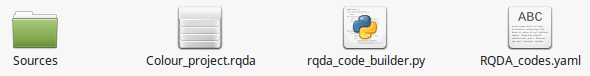
Create a directory as a parent for the project and open a command shell in it. Within the parent directory create a Sources directory. Place the source files in the Sources directory. In this example you can see two source files but typically this would be many files associated with interviews, observation logs, etc..

  $ mkdir Sources
  

  $ ls Sources
  Colours_of_Health_and_Sickness_Sociocult.txt
  Psychological_Properties_Of_Colours.txt
  

Run the 'R' program.

  
  $ R --quiet
  
  >
  

Add the RQDA library

Add the RDQA() library, this is the program that allows the researcher to analyse the data.

  
  > library(RQDA)
  Loading required package: RSQLite
  Loading required package: gWidgetsRGtk2
  Loading required package: RGtk2
  Loading required package: gWidgets
  Loading required package: cairoDevice
  Loading required package: DBI
  
  Use 'RQDA()' to start the programme.
  

The graphical tool starts.

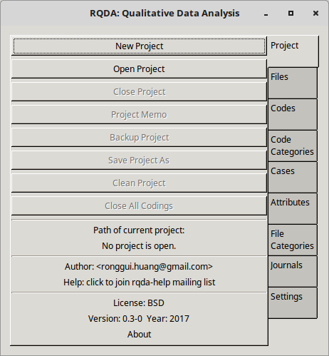
Create a Project

In the Graphical User Interface (GUI):

• Click New Project.
• Enter a name in the desired path: Colour_project.rqda. - Click OK.

A new project file appears in the directory.

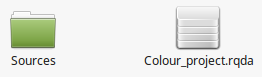
You may also notice in the R shell that the following command is executed.

  > [1] "~/Colour_project.rqda"
  

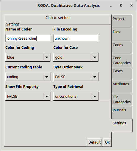
Name the coder

Select the Settings tab and define the Name of Coder in the first box.

Import source files to the project

The next step is to import source data. This can be achieved either through the GUI one by one, or in bulk using the R function write.FileList() in the R shell.

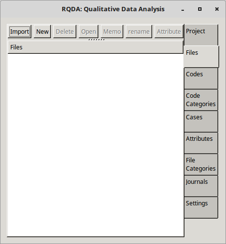
Using the GUI

To use the GUI, select:

• The Files tab followed by the Import button.
• Browse to each file in turn and select.
  

Using the R shell

An alternative mechanism is to use the R shell. This command using the addFilesFromDir() function selects the files in the Sources directory that match the pattern. In this case all files that end in the pattern .txt.

Execute the command:

  > addFilesFromDir('Sources', pattern = "*.txt$")
  

If you now check the GUI by clicking the Files tab, you will notice that the files from the Sources directory have been imported. Alternatively use the getFiles() function in the R shell to confirm.

  > getFiles()
  [1] "Colours_of_Health_and_Sickness_Sociocult.txt"
  [2] "Psychological_Properties_Of_Colours.txt"     
  attr(,"class")
  [1] "RQDA.vector" "fileName"
  

Coding

Inductive approach

RQDA() is very suitable for the inductive approach however it takes significant time.

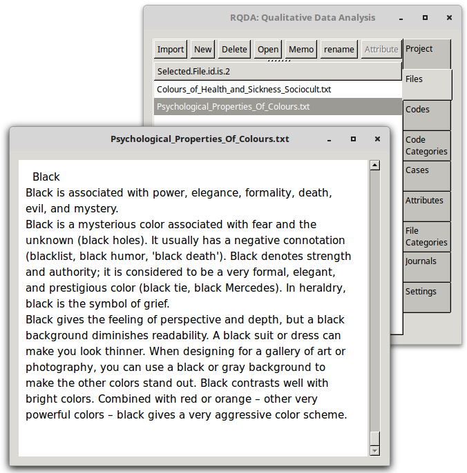
Select each document in turn from the Files tab, a popup appears with the text from the source file selected.

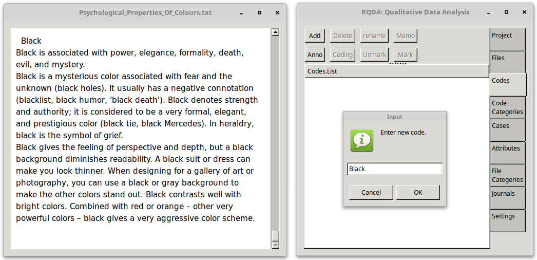
On the main GUI click the Codes tab and as a line is read that requires coding select Add and create the code. For example, to add a code Black, click Add. Enter the new code in the box provided and click OK. With text highlighted, select the appropriate code, i.e. Black and click Mark.

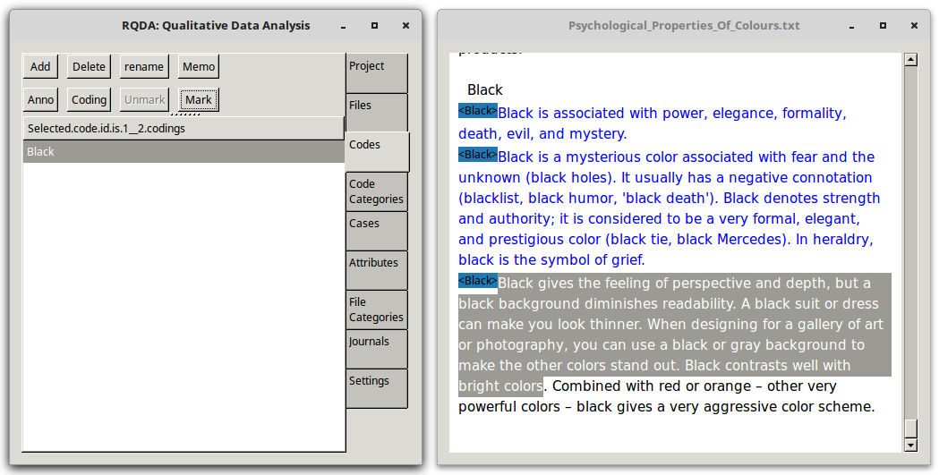
As can be seen each line is tagged.

Deductive approach

Unfortunately there does not appear to be a mechanism to import codes into the RQDA() database in bulk. For the deductive approach a researcher may have tens or even hundreds of categories and codes, it could be necessary to bulk upload. Extract the files from the RQDA-Code-Builder_v1.4.tgz which will give all the files including the database from this example as well as the rqda_code_builder.py. Move this file to the parent directory of the Sources directory.

The RQDA Code Builder (rqda_code_builder.py) program resolves this.

YAML file

YAML Ain't Markup Language (YAML) is a human-readable data serialisation language that is commonly used for configuration files, but can be used in many applications where data is being stored or transmitted. It is an ideal format for mapping of categories and codes.

The example project demonstrates how to deduct the following code schema as a YAML file in the same directory:

  $ cat RQDA_codes.yaml
    RQDA_codes.yaml
    ---
  
    Colour: 
     -  'Red'
     -  'Green'
     -  'Yellow'
     -  'Grey'
     -  'Black'
     -  'White'
     -  'Black'
     -  'Blue'
     -  'Pink'
     -  'Brown'
     -  'Purple'
  
    Psychological Properties:
     -  'Physical'
     -  'Intellectual'
     -  'Emotional'
     -  'Balance'
     -  'Spiritual'
  
    Floral Metaphors:
     -  'Daisy'
     -  'Juicy'
     -  'Apple'
     -  'Berry'
     -  'Flower'
     -  'Peach'
  
    Human Characteristics:
     -  'Divinity'
     -  'Eternity'
     -  'Infinity'
  

Executing the RQDA Code Builder

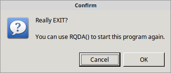
Before executing the RQDA Code Builder it is important to shut down the RQDA() application by clicking on the X in the top right corner and selecting OK to the Really EXIT? question.

The file that the RQDA() program uses to store data is an SQLite database. It is the file that was created at the beginning when the project was opened (Colour_project.rqda). The RQDA Code Builder reads the YAML formatted schema and uploads it to the database. It also creates a Structured Query Language (SQL) log of each SQL command it executes and more importantly develops a set of R commands that match text blocks to the codes. It has the following switches:

  -c|--coder [Name]   - Define coder, must match that from RQDA() settings.
  
  -d|--database [DB] -  Define path to SQLite3 database file.
  
  -y|--yaml [YAML]   -  Define path to YAML code file.
  

Execute the command, check it is version 1.4 or greater and execute with the relevant switches as demonstrated.

  $ cat rqda_code_builder.py | grep '# Version' | awk {'print $4'}
    1.4
  
  $ ./rqda_code_builder.py -c JohnnyResearcher -d Colour_project.rqda -y RQDA_codes.yaml
  
  
  RQDA Code Builder
  ----------------- 
  
  Connecting to the SQLite3 database Colour_project.rqda.
  Connected to the SQLite3 database Colour_project.rqda. Uploading..
  
  Upload completed
  ----------------
  
  A full list of SDL commands executed can be seen in the 'RQDA_SQL.log' file.
  You can restart the RQDA() library with the following command in the R shell:
  
  > RQDA()
  

Restart RQDA() as instructed.

  > RQDA()
  

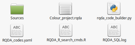
Two new files are created, RQDA_SQL.log which is a log of the SQL commands executed on the database as well as RQDA_R_search_cmds.R which is a list of commands that will be executed in the R shell to apply the deductive codes to the source files.

Applying the RQDA 'R' search commands

To apply the RQDA search commands execute the following command in the R shell. This bulk executes the commands in the RQDA_R_search_cmds.R file on all the source files.

  > source('RQDA_R_search_cmds.R')
  

Reviewing Coding

Before diving into the coding within the various source files, review the coding statistics. It can be seen from this extract that 385 code blocks were applied to the source texts.

  > getCodingTable()
      rowid cid fid     codename                                     filename
  1       4   1   2     Physical      Psychological_Properties_Of_Colours.txt
  2       5   1   2     Physical      Psychological_Properties_Of_Colours.txt
  3       6   1   2     Physical      Psychological_Properties_Of_Colours.txt
  4       7   1   2     Physical      Psychological_Properties_Of_Colours.txt
  5       8   1   2     Physical      Psychological_Properties_Of_Colours.txt
  6       9   1   2     Physical      Psychological_Properties_Of_Colours.txt
  
  ...   ...  ..   .    ...       ...
  
  378   381  22   2       Purple      Psychological_Properties_Of_Colours.txt
  379   382  22   2       Purple      Psychological_Properties_Of_Colours.txt
  380   383  23   1     Divinity Colours_of_Health_and_Sickness_Sociocult.txt
  381   384  23   1     Divinity Colours_of_Health_and_Sickness_Sociocult.txt
  382   385  24   1     Eternity Colours_of_Health_and_Sickness_Sociocult.txt
  383   386  24   1     Eternity Colours_of_Health_and_Sickness_Sociocult.txt
  384   387  25   1     Infinity Colours_of_Health_and_Sickness_Sociocult.txt
  385   388  25   1     Infinity Colours_of_Health_and_Sickness_Sociocult.txt
      index1 index2 CodingLength
  1      399    534          135
  2     4109   4197           88
  3     4739   4842          103
  4      848    977          129
  5     1454   1587          133
  6     4257   4394          137
  
  ...   ...     ...          ...
  
  378  15568  15620           52
  379  15621  15663           42
  380   3189   3301          112
  381  15902  16020          118
  382   3189   3301          112
  383  15902  16020          118
  384   3189   3301          112
  385  15902  16020          118
  

Reviewing the coded blocks

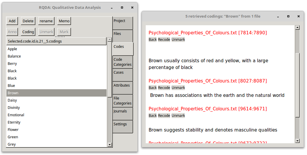
Selecting the Codes tab from the RQDA() GUI and select any particular code. In this case Brown was selected. Click on the Coding button and a popup appears with each instance of sentences within the source files where the word Brown or brown appeared, such sentences were tagged with the Brown tag. The popup also shows for each block the source file from where the sentence appeared.

This performs an initial deductive coding. There may be quirks however, what if one interviewee kept referring to Beige but the researcher wanted to code it as Brown? or the researcher has a code Colour and some of the transcripts were transcribed in American English. In this case sentences with Color should be coded with Colour.

Carry out additional coding of sentences like this.

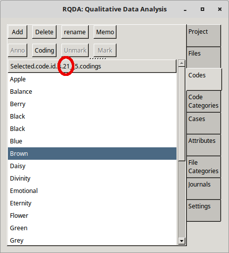
First find the CID of the Code for Brown. Select the Codes tab, click on the Brown code and its CID can be seen at the top of the pane as shown by the red circle in the diagram.

Execute the following two lines in the R shell and they will be added to the main coding already performed.

  > codingBySearch("Beige",fid=getFileIds(),cid=21,seperator="[.!?]")
  
  > codingBySearch("beige",fid=getFileIds(),cid=21,seperator="[.!?]")
  

Visualising categories

There are some tools built into RQDA() for visualisation. For example using the D3.js JavaScript library for manipulating data. D3 helps bring data to life visually using Hypertext Markup Language (HTML), Scalable Vector Graphics (SVG), and Cascading Style Sheets (CSS).

Installing d3Network

On the R Shell install D3.js and activate the d3Network within R.

  > install.packages('d3Network')
  
  > library(d3Network)
  

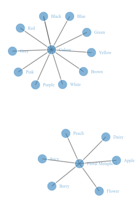
Visualising Categories

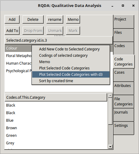
Select the Categories tab, highlight a Category or many Categories using the ctrl button and right click. Scroll down to the Plot selected code categories with d3. A HTML page will popup with diagrams like these:

Summary

There are a lot more features to R and RQDA() that can aid qualitative research. The additional RQDA Code Builder program (rqda_code_builder.py) allows the researcher to deductively pre-build a code schema and apply it automatically.